matrix conventions

Matrix transformations are very powerful and useful in computer graphics. But they can be tricky to get right. This article won’t talk about the detailed mathematics of matrices—you can find plenty of descriptions of that elsewhere—but about the practicalities of getting matrix transformations correct in your program code.

First of all, let me offer two important rules when writing matrix-manipulation code:

Rule 1: Pick a convention and stick to it. There are two self-consistent ways to write down a matrix transformation that takes a vector in object space (the coordinates in which the object is defined) and transforms it to world space (the coordinates in which the object is viewed): either as post-multiplication on a row vector, e.g.:
```
 object-space vector → matrix1 → matrix2 → world-space vector
```
or as pre-multiplication on a column vector, e.g.:
```
 world-space vector ← matrix2 ← matrix1 ← object-space vector
```
It may look like the first form is more natural (the transformation sequence going left-to-right rather than right-to-left), but in fact most code uses the latter, and it is probably the more convenient form for trying to envision what is going on, as we will see shortly. But the most vital thing is to be absolutely clear which convention is in effect.
Rule 2: Understand, don’t fiddle. If your transformations are coming out wrong, don’t try randomly fiddling with the order of the components to get them right. You might succeed eventually, but it is quite possible that you made two mistakes somewhere that just happen to cancel out. While two wrongs may make a right in this case, you have set a trap for yourself if you (or someone else) have to make an adjustment later: you might try to change the angle of a rotation, for example, only to discover that it has the opposite effect from what you expected; or your x-and y-scaling might be the wrong way round. So always try to understand why your transformations are in the order they are. The effort spent up-front will help keep things less confusing later on.

Now let me give a handy tip for trying to envision the effect of a sequence of matrix transformations. Assuming the usual pre-multiplication-of-column-vectors convention, we can imagine each matrix as a magic box that, when we look through it, transforms the appearance of space on the other side, making things bigger or smaller, rotating or repositioning them and so on. So if we represent object space by the object we are looking at (here a simple line-drawing of a teapot), ahd world space by the eye of the observer, then a transformation like

world-space vector ← matrix ← object-space vector

can be visualized as

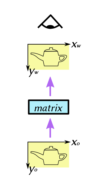
where the purple arrows show the flow of geometric information from object space (coordinate system (x_o, y_o)), through the matrix transformation box, to the observer’s eye (coordinate system (x_w, y_w)).

The basic principles apply equally to both 2D and 3D graphics. Here we are dealing with 2D graphics in Cairo. The examples will be in Python, using the high-level Qahirah binding. This lets us represent the transformation of a Vector object by a Matrix object directly as a simple Python expression:

user_space_coord = matrix * object_space_coord

Let us envision what happens if we apply a simple rotational transform to the object.

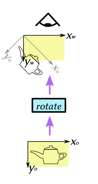
By superimposing both coordinate systems in the upper part of the diagram (the current one in black, the previous one in grey), we can see the differing effects of, for example, moving parallel to the axes in object space coordinates (x_o, y_o) versus world space coordinates (x_w, y_w). In the Python code, we can spread things out across multiple lines, to more closely approximate the arrangement in the diagram:

user_space_coord = \
    (
        Matrix.rotate(45 * deg)
    *
        object_space_coord
    )

Now, what happens if we apply two transformations in succession?

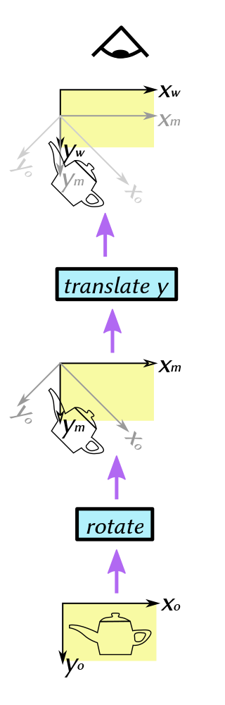
Here the transformations (in order from object space to world space) are rotation about the origin, followed by translation along the positive y-axis. The rotation converts from object coordinates (x_o, y_o) to the intermediate coordinate system (x_m, y_m). The translation then converts from (x_m, y_m) to (x_w, y_w) coordinates. The equivalent Python code would be something like

user_space_coord = \
    (
        Matrix.translate((0, 10))
    *
        Matrix.rotate(45 * deg)
    *
        object_space_coord
    )

Here the order is reversed, the y-axis translation being applied first:

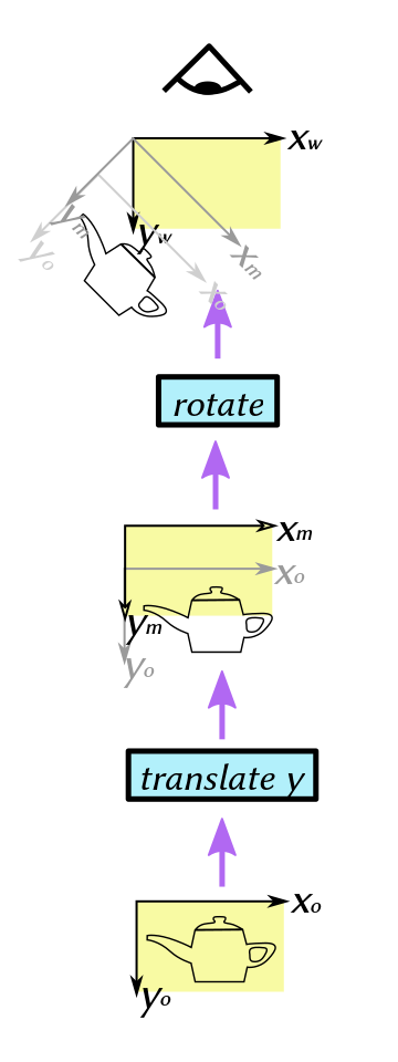
Thus, the rotation takes place, not about the (x_o, y_o) origin, but about the (x_m, y_m) origin.

Each transformation (blue background) is applied in the coordinate system of the picture of the object immediately below it (yellow background).

Note that, while the orientation of the teapot ends up the same in both these cases, its position is different. The equivalent Python code would be correspondingly rearranged to match the diagram:

user_space_coord = \
    (
        Matrix.rotate(45 * deg)
    *
        Matrix.translate((0, 10))
    *
        object_space_coord
    )

So, when you look at the Python code, imagine the eye of the observer on the receiving end of the value of the expression, at the top, while the object coordinates are at the bottom, being processed through successive stages of the transformation until they get to the top. Each individual Matrix object corresponds to one of the boxes with a blue background, while the multiplication asterisk immediately below it corresponds to the picture with the yellow background immediately below that box.